5 Data Inputs
- stressor_response_demo.xlsx
- stressor_magnitude_demo.xlsx
- watersheds.gpkg
- life cycles.csv
5.1 Stressor-Response Workbook
5.1.1 Purpose
The stressor-response workbook contains all the stressor-response curves applicable to a target study system (e.g., Athabasca Rainbow Trout). These stressor-response curves are used within the CEMPRA (Joe Model) tool to predict cumulative effects additively given stressor magnitude values (discussed in the next section). Stressor-response functions can also be linked to specific vital rates in the life cycle model.
5.1.2 Layout
The stressor-response workbook is an Excel workbook containing all stressor-response functions to be used in the CEMPRA (Joe Model). The first worksheet contained within this Excel workbook must be titled “Main”. This worksheet is used as a coversheet to describe and organize each of the stressor-response curves. Subsequent worksheets describe each of the stressor-response functions relevant to a particular species, where each stressor-response function has its own worksheet. Note that the spelling of the stressor name must be identical between the “Stressors” column in the “Main” worksheet and the worksheet title (on the bottom tab) for each stressor.
Work is currently underway to develop an online stressor-response web database (a digital repository of stressor-response functions across species, systems and geographic areas compiled across reference literature). As this database grows, functionality will be expanded to automatically generate a stressor-response workbook of selected stressors using the R-package (CEMPRA). See details in Appendix A.
5.1.2.1 Main Worksheet
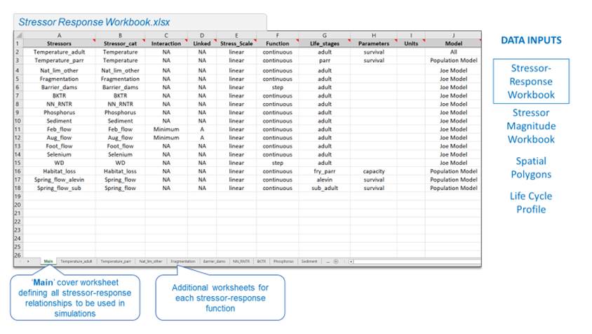
Figure 5.1 shows the main worksheet in the Stressor-Response workbook.
The purpose of the “Main” worksheet is to organize and summarize stressor-response functions within the workbook. The columns within this worksheet are set up as follows. Inputs must be diligently followed in order for the code to work:
| Column Name | Description |
|---|---|
| Stressors | Name of the stressor. This must match the stressor-response worksheet title. It must also match the “Stressor” column in the stressor magnitude workbook. Avoid the use of spaces in stressor names. |
| Stressor_cat | Category of the stressor. Only relevant if multiple stressors are linked with a defined interaction. If there is no interaction, simply copy the stressor name here. |
| Interaction | Min/max interactions between stressors. Set to NA or leave blank if there are no interactions. Possible interactions available include “Minimum” or “Maximum”. If multiple variables are linked together with “Minimum”, the variable with the lowest stressor-response score in the Joe Model will be used, and the other variables will be omitted from the CEMPRA (Joe Model) calculation. For example, consider road density and stream crossings (link these together with a Minium interaction to avoid double-counting highly correlated stressors). Once set, determine which stressors should then be linked together by defining groups in the “Linked” column. Use letters A, B, C etc., to define distinct groups. If no special interaction is defined between variables, then set these cells to NA. |
| Linked | For Variable Interaction Linkages: Use NA if no interaction is defined for the target variable; otherwise, choose letters A, B, C, D etc. to specify variable groups. For example, if there were four stressor-response curves for July, August, September flows (highly correlated in some systems), and they were encoded as three separate stressors, users could apply the “Minimum” interaction function to link the lowest system capacity across all four terms but only have one summer flow SR function in the CEMPRA (Joe Model). In this case, the letter A would be used to group all these terms together. |
| Stress_Scale | Stressor Scale can be either “linear” or “log” to specify a linear or logarithmic function, respectively, for interpolation (in raw units of the stressor). |
| Function | Either “continuous” or “step”. “Continuous” will apply linear interpolation between values, and “step” will adjust mean system capacity values in discrete steps (e.g., number of barriers). |
| Life_stages | (Only relevant for the Population Model) Which life stage should each stressor be linked to? Set all values to “adult” if unspecified. The default assumption in the Joe Model is that stressor-response curves are linked to “adult” system capacity. stage_e: eggs (linked to the egg to fry transition) stage_0: sub-yearling (linked to the sub-yearling (Age-0) age class. For example, fry or alevin) stage_1: yearling age class (e.g., parr, age-1 to age-2 transition). stage_2: stage 2 class (i.e., stage-2 to stage-3 transition). stage_3: stage 3 class (i.e., stage-3 to stage-4 transition). stage_x…: stage … class (i.e., stage-(x) to stage-(x+1) transition). stage_Pb_1: (anadromous only) applies to age-1 (yearlings/parr) pre-breeder (Pb) class. stage_Pb_2: (anadromous only) applies to age-2 pre-breeder (Pb) class. stage_Pb_3: (anadromous only) applies to age-3 pre-breeder (Pb) class. stage_Pb_…: (anadromous only) applies to age-x pre-breeder (Pb) class. stage_B_2: (anadromous only) applies to age-2 spawners (B-breeder) class. stage_B_3: (anadromous only) applies to age-3 spawners (B-breeder) class. stage_B_4: (anadromous only) applies to age-4 spawners (B-breeder) class. stage_B_x…: (anadromous only) applies to age-x spawners (B-breeder) class. spawners: (anadromous only) applies to all spawner age classes. u: (anadromous) applies to ALL spawning age classes, generally controls the global prespawn survivorship. u_3: (anadromous) applies to age-3 prespawn survivorship. u_4: (anadromous) applies to age-4 prespawn survivorship. u_…: (anadromous) applies to age-x prespawn survivorship. smig: (anadromous) applies to ALL spawning migration age classes, generally controls the global spawning migration survivorship. smig_3: (anadromous) applies specifically to age-3 spawning migration survivorship. smig_4: (anadromous) applies specifically to age-4 spawning migration survivorship. smig_…: (anadromous) applies specifically to age-x spawning migration survivorship. |
smig: (anadromous) applies to ALL spawning migration age classes, generally controls the global spawning migration survivorship.
smig_3: (anadromous) applies specifically to age-3 spawning migration survivorship.
smig_4: (anadromous) applies to age-4 spawning migration survivorship.
smig_…: (anadromous) applies to age-x spawning migration survivorship.
If you are making use of the integrated life cycle model, then possible life stages include “SE” for eggs and “S0” for hatchling/fry. Both SE and S0 are Age-0 individuals. For subsequent stages, use “stage_1”, “stage_2”, “stage_3” etc. for stage-specific linkages (see Section 6.4 and Section 8 for clarification).
If the same stressor is linked to multiple life stages, special terms such as “sub_adult” or “adult” can be used to define linkages to all immature (Age-1+) stage classes and all mature (Age-1+) stage classes, respectively. The term “all” will mean that the stressor response curve is linked to all life stages.
If the same environmental variable is linked to different life stages with different stressor-response curves, then it is recommended that the user duplicate stressor values and treat them as distinct environmental variables to avoid confusion (e.g., “Temperature_adult”, “Temperature_parr”). | | Parameters | Only relevant for the integrated life cycle model: leave blank for scenarios that only make use of the Joe Model.
If the stressor-response function is being linked to a vital rate in the life cycle model, describe how the stressor-response curve is linked to the life stage (which vital rate is affected). This column can be left blank if a user is only interested in running the Joe Model.
Possible mechanisms include “capacity”, “survival,” or “fecundity”. Once set, the response component of the stressor-response curve will act as a multiplier to the specified vital rate. For example, if a stressor is linked to “survival” of stage X and the stressor-response curve estimates a scaled response of 0.8 based on the stressor magnitude, then the default baseline survivorship will be multiplied by 0.8 in the simulation (e.g., original survivorship of life stage X: 0.34; adjusted survivorship of life stage X: 0.80.34 = 0.27).
• survival: Stressors linked to “survival” modify the default survivorship of a given life stage transition.
• capacity: Stressors linked to “capacity” will modify the stage-specific capacity values by a multiplier (0 – 1) based on the stressor-response relationship, regardless of the mechanism used to represent density-dependent constraints on growth (compensation ratios vs location and stage-specific K values, See Section 8). Capacity adjustments will be implemented as the final step in the calculation. Stressor-response functions linked to capacity will only have an effect if the life stage is parameterized with density-dependent constraints (e.g., compensation ratios ≠ 1.0 or Beverton-Holt K values enabled). If a stressor-response function is linked to a life stage, but there are no density-dependent constraints on that life stage in the life cycle profile, then the stressor will not have an effect on the simulation.
• fecundity: Stressor-response functions linked to fecundity will adjust the (eps) eggs per spawner (female) using the response value as a multiplier on the default input fecundity. For example, if the default fecundity is 3,000 and a stressor linked to fecundity has an effect of 0.6 (response), then the resulting fecundity (epf) in the life cycle model will be 3,000 0.6 = 1,800. Note that the stressor-response relationships must be linked to a sexually mature life stage for the fecundity multiplier to be meaningful. For example, if a fecundity multiplier is linked to an early life stage (e.g., stage_1), but the target species does not become mature until stage_3, then the stressor will have no observable effect on the population.
Response (effect) estimates from the stressor-response curves will always be adjusted to 0 if biological response values are below zero, and adjusted to 100 (1.0) if response values exceed 100% in the stressor-response workbook. This ensures that survivorship remains between 0 and 1. | | Units | Optional: include units as meta data (a friendly reminder). This column is not used in any calculations but is included as metadata and displayed on summary plots in the tool (where available). | | Model | Set all values to “Joe Model” if not using the life cycle model.
This column is used to define which assessment endpoint the stressor-response curve should be applied to. Possible options include “All”, “Joe Model,” or “Life cycle model”. “All” specifies that the stressor-response curve is generic enough to be used in both the Joe Model and the life cycle model. “Joe Model” specifies that the stressor-response relationship should only be used in the simplified Joe Model roll-up summary. “Life cycle model” specifies that the stressor-response relationship is only applicable to the life cycle model. |
5.1.2.2 Individual Stressor-Response Curve Worksheets
The remaining worksheets in the Stressor-response workbook are all used to describe the relationships between raw stressor values (on the x-axis) and the biological response (on the y-axis) (i.e., the stressor-response data).
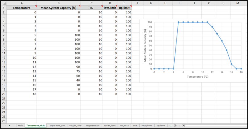
- Example of an individual stressor worksheet within the stressor response Excel workbook.
Individual stressor worksheets within the stressor-response file contain stressor-response curves for each of the stressor-response functions outlined in the “Main” worksheet (one worksheet for each row). The spelling of the worksheet name must exactly match the spelling of the stressor on the ‘Main’ worksheet. Additional rows can be added (as needed) to increase the resolution and specify the shape of a complex non-linear stressor response curve. Threshold stressor-response functions or stressor-response functions with discrete values may have relatively few rows.
The columns within each stressor-response worksheet are formatted as follows:
| Column Name | Description |
|---|---|
| [Stressor] | The raw value of the stressor (on the x-axis). For example, the temperature would likely be valued in degrees Celsius, but the units and additional metadata are declared on the ‘Main’ worksheet. |
| Mean System Capacity (%) | The Mean System Capacity (on the y-axis) is associated with the raw stressor value on the x-axis. This column is the response component of the stressor-response curve. Values should be entered as a percentage and range from 0 to 100. Note that, for the life cycle model, this value may be the life-stage-specific dose-response curve for capacity or survival. Mean system capacity is user as a generic term across the Joe Model and Life Cycle Model. |
| SD | Standard Deviation (SD) is used to resample the mean system capacity (response) values based on a given stressor level. In the CEMPRA (Joe Model) simulations, environmental parameters are resampled for each batch replicate, year and location based on SD values in the stressor magnitude workbook. This column is used to represent uncertainty in the stressor-response relationship. Resampling will be based on the mean system capacity and SD values with a normal distribution (linear) or log scale (log) according to the value specified in the main worksheet under the Stress_Scale column. Regardless of the parameters for resampling, the lower limit and upper limit values will constrain values to fixed limits. If the SD value is set to zero, then no resampling will take place within the stressor-response curve. |
| low.limit | The lower limit for stressor-response resampling (see SD column distribution). Set to 0 as a default. |
| up.limit | The upper limit for stressor-response resampling (see SD column distribution). Set to 100 as a default. |
5.1.3 How to Build Your Own Stressor-Response Function
CEMPRA (Joe Model) users can either select pre-assembled stressor-response functions or define their own stressor-response functions for use in the model. A library is currently being developed to host pre-assembled stressor-response functions and their associated documentation (Appendix A). Users who develop their own stressor-response functions are encouraged to fill out the appropriate documentation for their function and upload it to this public stressor-response library for future use (Appendix A). Please see (MacPherson et al., 2020) and (Rosenfeld et al., 2022) for further discussion on fundamental considerations in the development of customized stressor-response functions.
5.1.3.1 Methodology
Depending on data availability, stressor-response functions may be developed from available empirical data, from the elicitation of experts and stakeholders, or from existing literature.
When using empirical data, the response component of the stressor-response relationship must be standardized to a common response metric. For convenience, the CEMPRA tool uses Mean System Capacity as a generic nickname to represent a standardized response scaled from 0% to 100%. In the CEMPRA tool (both the Joe Model and Life Cycle Model assessment endpoints), stressor-response relationships are reported as a scaled response value from 0% to 100%. These values are reported in the stressor-response workbook. The default assumption is that when a stressor is at its lowest level (or least harmful state if the scale is reversed), the mean system capacity will be set to 100% for that stressor. If this adjustment is not made, scenarios will be ranked differently simply by including specific stressors for comparison regardless of ecological state.
5.2 Stressor Magnitude File
5.2.1 Purpose
The stressor magnitude file is an Excel worksheet which defines and bounds each stressor within the individual locations (i.e., spatial units) being assessed. Similar to the stressor-response functions, stressor magnitude values are sampled across locations with stochasticity. The stressor magnitude workbook is structured accordingly, with data for each stressor and location entered into the dataset in a long table format (as opposed to the standard wide table format). Each row specifies a unique stressor for each unique location. Therefore, the number of rows in this dataset should be equal to the number of stressors multiplied by the number of locations. For each simulation in the CEMPRA tool, values are sampled at random with stochasticity for each stressor and location. For each year and batch replicate, stressor magnitude values will be drawn from each normal (or lognormal) distribution based on the Mean and SD (standard deviation) and then further constrained based on the specified lower and upper limits.
If there is no suspected uncertainty or interannual variability in stressor magnitude values for a given stressor and/or location, then the SD value can be set to 0, and the lower limit, upper limit and distribution type can be ignored.

5.2.2 Layout
Each row in the stressor magnitude workbook specifies a relationship between a unique stressor and a unique location. Locations (discussed in detail in the next section) are specified by a unique ID (HUC_ID) and NAME. The HUC_ID column is a legacy from an older version of the Joe Model that referenced Hydrological Unit Codes as ID values, but HUC_ID can be any set of unique IDs specified by the user for their spatial units of interest. The NAME column can be blank but is included for convenience since many users find it challenging to cross-reference ID values between different datasets.
| Column Name | Description |
|---|---|
| HUC_ID | An ID field is used to represent a unique location (spatial unit). The HUC_ID column is a legacy from an older version of the Joe Model that referenced Hydrological Unit Codes as ID values, but HUC_ID can be any set of unique IDs specified by the user for their spatial units of interest. The NAME column can be blank but is included for convenience since many users find it challenging to cross-reference ID values between different datasets. The HUC_ID field must match the feature column HUC_ID in the spatial polygons file. |
| NAME | The NAME of the polygon in the spatial polygons file. This field must match the NAME column in the spatial polygons file, but it can be blank if a spatial unit does not have a defining name. |
| Stressor | Stressor Name. This must match the information and sheet names in the stressor-response workbook. |
| Stressor_cat | Name of the Stressor category. This column must match the spelling used in the stressor-response workbook. |
| Mean | The mean value of the stressor for the spatial unit (location) HUC_ID (polygon). |
| SD | Standard deviation (SD) of stressor values for the target HUC_ID. During the simulation, stressor values for each HUC_ID are resampled from a distribution with mean and SD values. Setting the SD to zero means that there will be no variability in the stressor value during the simulation. |
| Distribution | Type of distribution to use for resampling. Either “normal” or “lognormal”. We recommend using a “normal” distribution where possible. Testing coverage is incomplete for “lognormal”. |
| Low_Limit | The lower limit for resampling. |
| Up_Limit | The upper limit for resampling. |
| Comments | Internal comments by the user for personal reference. It can be blank. |
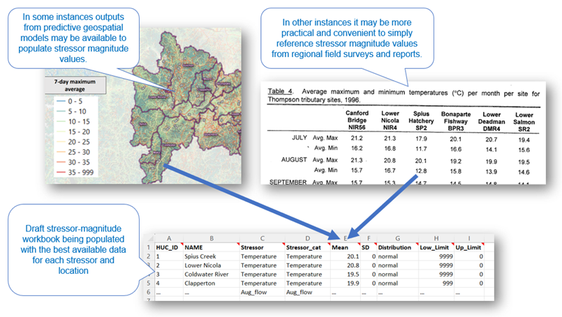
5.2.3 Assembling Your Own Stressor-Magnitude Data
Data for stressor magnitude estimates can come from a variety of sources, including GIS data, modelled data, field data, expert opinion, regional trends, or estimates from the literature. When assembling your own stressor magnitude data, stressor magnitudes and ranges will need to be assigned to the individual locations (spatial units) being represented in the model. Stressors within each location must be assigned a magnitude, and distribution or the SD value must be set to 0 for simulations with no stochasticity. Within each spatial unit, users can specify the mean value, standard deviation, distribution (normal or lognormal), and upper and lower limits of each stressor, as discussed in the previous section.
Stressor magnitude values should be aggregated to locations to represent location-averaged estimates. Locations can be split and aggregated as needed such that each location represents averaged generalized conditions.
5.3 Locations (Spatial Polygons)
Locations are represented in the CEMPRA tool as spatial polygons. Locations should be defined to reflect heterogeneity in stressor values across the study area.
Spatial polygons are imported into the CEMPRA tool as a GIS data file. Possible formats include either geopackage (.gpkg) or shapefile (.shp) format. The spatial units GIS data file does not contain any stressor magnitude data for modelling but consists of just the geometry and fields for the location ID (HUC_ID) and NAME. The polygon geometry included in this file is used for display purposes only and is joined to the stressor magnitude file when imported into the CEMPRA. Therefore, the size and shape of each spatial unit do not influence any components of the assessment.
Regardless of the file format, the GIS (locations) spatial polygon data file must meet the following criteria:
- “HUC_ID” field: The locations data layer must have an attributed field labelled ‘HUC_ID’ with a unique identifier for each spatial unit (location).
- “NAME” field: The locations data layer must have an attributed field labelled ‘NAME’. This field is included for convenience. Values in this field can be blank, but users are encouraged to populate this field.
- The HUC_ID and NAME fields must match values (and spelling) in the stressor magnitude Excel input so data can be cross-referenced and joined in the tool.
- The spatial polygons file must be imported in the standard latitude/longitude projection (CRS: “EPSG:4326 – WGS84”). External GIS software such as QGIS can be used to transform projections as needed.
- There should be no geometry errors (invalid geometries) in the polygon geometry data. Run check geometry and fix errors in programs such as QGIS.
- Simplify geometries: we recommended running functions like ‘Simplify geometries’ in programs such as QGIS to reduce the file size before importing data into the CEMPRA tool. Ideally, the locations spatial polygon data file should be under 10MB for the best performance in the Shiny application. Processing larger datasets is possible by using the R package version of the CEMPRA tool.

5.4 Life Cycles Profile
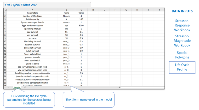
The life cycle profile (csv file) is an optional input applicable to users who are interested in running the integrated life cycle model. The life cycles profile file specifies all input parameters required to run the life cycle model (e.g., number of stages, survival rates, fecundity, etc.). The format of the life cycles profile is a generic template, but once populated, it is used to parameterize the life cycle model for a specific study system. Usually, this consists of a target population (e.g., Athabasca Rainbow Trout, Nicola Basin Chinook Salmon, etc.).
- “Parameters” field: Nickname for parameter. Can contain any text defined by the user.
- “Name” field: Target name field used by code in the population model. Inputs here are restricted.
- “Value” field: Input value for parameter Name.
See chapter on the life cycle model for further details.
A detailed discussion of the life cycles profile (csv file) is included in Section 8.2 with accompanying background information. It’s possible to run the Joe Model and omit the life cycle model entirely. Therefore, the life cycles profile csv should be considered as an optional input for advanced use cases of the CEMPRA tool.
Leave questions and comments below (via your GitHub account)