6 Joe Model & Shiny App – CEMPRA Guidance Document

6.1 About

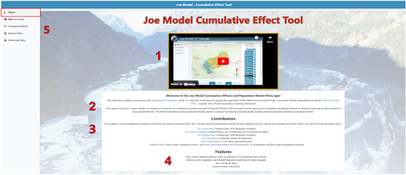
When you first access the R Shiny web application for the CEMPRA, you will be automatically directed to the About page. This page contains a brief introduction to the application and the CEMPRA (Joe Model) tool, a list of contributors, and a list of features for users to explore. A tutorial video is also embedded on this webpage to guide users through the application.

6.2 Upload Data

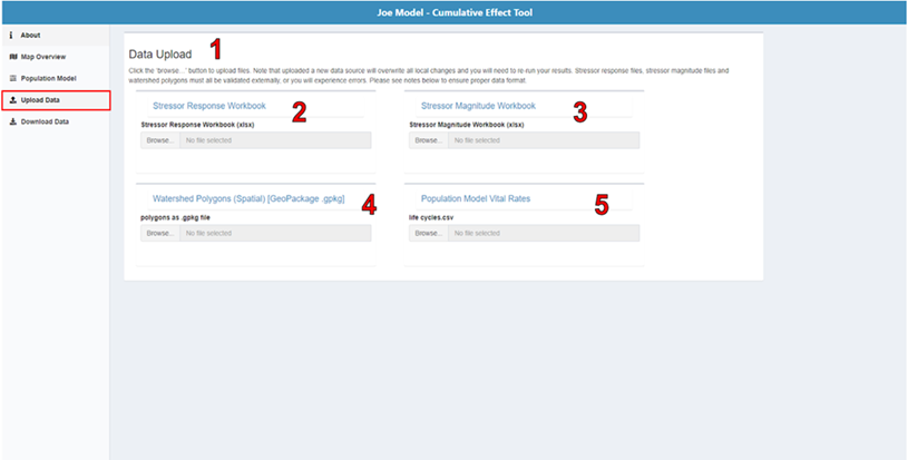
If you would like to import a custom set of stressor-response functions, spatial polygons, or vital rates (for the life cycle model), select the Upload Data page in the menu on the left side of the screen. This page allows you to upload four key input files from your computer: the stressor-response workbook (.xlsx), the stressor-magnitude workbook (.xlsx), a spatial polygons file (.gpkg or .shp), and a life cycle profile (.csv). To upload a file from your computer, click “Browse…” on the toolbar below the associated file heading. Next, select the desired file from the file window and click “Open”. The file will begin to upload. A status bar will appear below the file name, indicating the upload status. Once the file has been successfully uploaded, the status bar will display “Upload complete”.

Figure 6.2: Data upload page of the R Shiny web application. 1) Instructions for uploading files. 2) Location to upload stressor-response workbook (.xlsx). 3) Location to upload stressor magnitude workbook (.xlsx). 4) Location to upload spatial polygons file (.gpkg or .shp). 5) Location to upload life cycle profile (.csv).

6.3 Joe Model and Main Overview

6.3.1 Map Window

The map window on the Map Overview page allows users to view stressor magnitudes and model results in a choropleth map based on the spatial polygons layer you imported. The map in the centre of the screen is interactive and allows users to scroll, zoom, and select individual polygons. When hovering over a polygon, users will see the name and HUC_ID of that polygon displayed directly above the map window. To select a polygon, click on it once. Selected polygons will appear in blue. Clicking on additional polygons will add to your selection. To deselect a polygon, click it again. The number of selected polygons (HUCs) will appear below the map window on the left-hand side. Click the “deselect all” button beside this text string to deselect all polygons.

6.3.2 Stressors

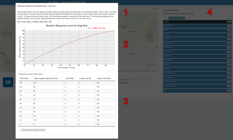
On the Map Overview page, users can view stressor-response relationships for each of the stressors included in the input stressor-response Excel workbook. A list of these stressors is on the screen’s right side. Clicking on the chart icon next to one of the stressors opens a pop-up window to view the stressor-response curve and raw stressor-response table associated with that specific stressor. You can edit cell values within the stressor-response table by double-clicking on the cell you want to edit. Any edits to the stressor-response table will automatically appear in the stressor-response curve.

Figure 6.3: Stressor-response relationship pop-up window example. 1) Description of table and stressor-response curve. 2) Stressor-response curve plot. 3) Stressor-response curve input table. 4) List of stressors used in the CEMPRA (Joe Model).

6.4 Joe Model Runs

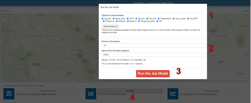
To run the Joe Model, click the “Joe Model” button in the centre of the lower panel. In the pop-up window, you can select/deselect variables that you want to include/exclude in the Joe Model run. In addition, you can specify the number of simulations or batch runs you would like to conduct (in the “Number of Simulations” box), and you can provide a name for the simulation (in the “Name of this Simulation” box). When you are ready to run the Joe Model for all spatial polygons in the study area, click “Run the Joe Model”. Note there is currently no option to run the Joe Model for individual spatial polygons.

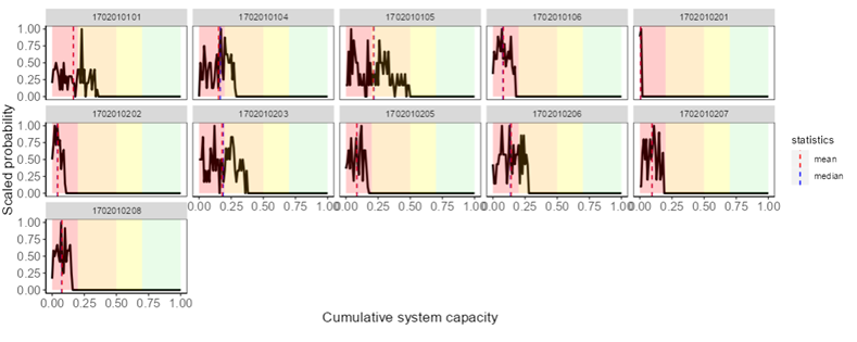
Figure 6.4: Pop-up window for the Joe Model. 1) Variables to include/exclude from cumulative effects modelling. 2) Inputs for the number of simulations and the name of the simulation. 3) Button to run the Joe Model. 4) Button to bring up the pop-up window.

6.4.1 System Capacity Plots

After running the Joe Model, a new section labelled “System Capacity Plots” will appear at the bottom of the map page. You can view tables and plots of the cumulative system capacity for selected watersheds (click “Selected watersheds”) or for all watersheds (click “All watersheds”) compared to the global mean system capacity across all simulations.

System capacity plots show the scaled probability output from the Joe Model from stochastic simulations.

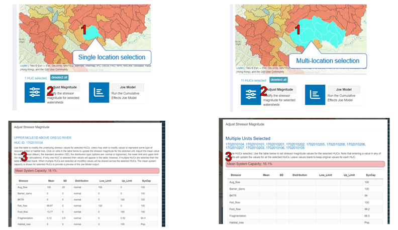
Figure 6.5: System capacity plots for eleven spatial units (locations) showing the cumulative system capacity scores (mean, median and scaled probability distributions).

6.5 Adjust Stressor Magnitude

Users may wish to modify stressor values to represent recovery action or habitat loss. To view and edit stressor magnitudes for an individual spatial polygon, select the spatial polygon of interest and click “Adjust Magnitude” on the right-hand side of the lower panel. Next, review the mean system capacity in the pop-up window for one or more selected locations. Below this, a table containing all the stressors, their magnitudes and distributions will be displayed. Double-click on the desired cell to edit any of the values in this table. Adjust the mean value for each stressor (Mean), the standard deviation (SD), the distribution type (options are normal or lognormal), and the lower limit and upper limit (for stochastic simulations). Note that stressor names and system capacity values cannot be edited. If only one HUC is selected, values will appear in the table; however, if multiple HUCs are selected, the table will appear blank. When multiple HUCs are selected, all modified values will be shared across the selected HUCs. The mean system capacity is shown for selected HUCs to preview the model output.

Figure 6.6: Example of single or multi-location stressor magnitude adjustment across spatial units.

6.6 Weighting Joe Model Result Scores

Several alternative methods are available to integrate or add up Joe Model Cumulative System Capacity Scores across locations:

Summary Method 1: Cumulative System Capacity Scores are Summarized Across Locations with Equal Weighting
Summary Method 2: Summarizing Cumulative System Capacity Scores Across Locations with a Locally Weighted Mean
Summary Method 3: Multiply Joe Model Response Scores and Another Metric (e.g., area × density) to Weight Results Across Locations

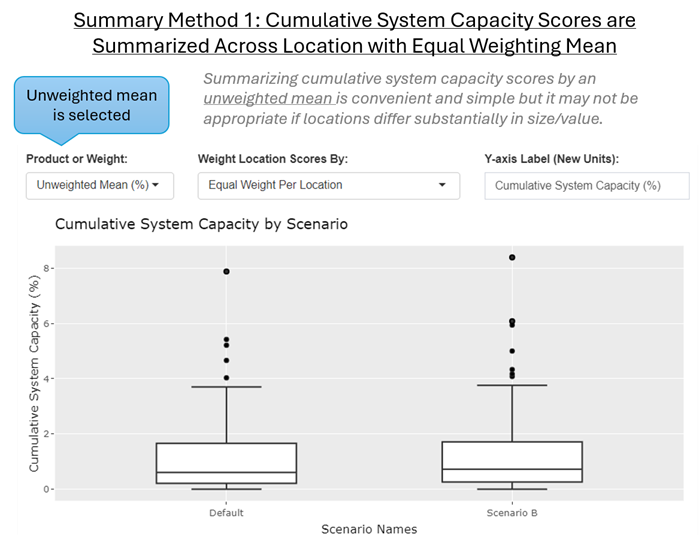
Summary Method 1: Cumulative System Capacity Scores are Summarized Across Locations with Equal Weighting

Overview: When Joe Model Cumulative System Capacity result scores are summarized across locations (i.e., reach, polygon) and scenarios, by default the average score is calculated as an unweighted mean across locations (i.e., each location is weighted equally). This is appropriate if locations can be weighted equally or are assumed to be of equal value, size, etc. However, if this is not the case, then Summary Methods 2 or 3 can be used to summarize values as a weighted mean, and/or by taking the product of the scores and another weighting variable.

Calculation Method: By default, Joe Model Cumulative System Capacity scores are summarized across locations with a simple unweighted mean. This is repeated for each MCMC batch replicate.

Applications: If all locations represent approximately equal sizes or values, then this method is appropriate. In many instances, the Joe Model is run with locations that represent standardized hydrological units (watersheds), defined by a Hydrological Unit Code (HUC, 1-12). When using standardized hydrological units an unweighted mean is appropriate. In British Columbia, the Joe Model is occasionally run with Assessment Watersheds from the BC Freshwater Atlas. The Assessment Watersheds approximately represent standardized location units so summarizing values across locations with an unweighted mean is appropriate. In other instances, summaries are completed across discrete units as a part of an inventory where size and weighting are irrelevant (e.g., when comparing or summarizing status of populations or watersheds that are of equal intrinsic value).

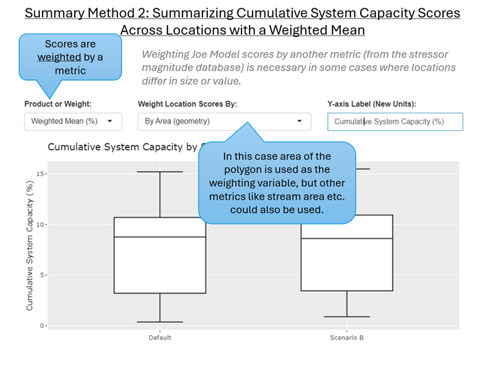
Summary Method 2: Summarizing Cumulative System Capacity Scores Across Locations with a Weighted Mean

Overview: In many instances, taking an unweighted mean will not be appropriate because locations differ considerably in size/value, or there is prior knowledge about habitat availability or weighting per location. For example, consider discrete watersheds that differ considerably in terms of their size and stream area. Additionally, consider instances where there is prior knowledge about the actual habitat availability within a location. Where possible we want to adjust Joe Model Cumulative System Capacity Scores so that the final value reported across locations is weighted by an appropriate metric such as habitat area which will represent a proxy for local population size or habitat capacity.

Calculation Method: We can choose to summarize system capacity scores with a weighting variable. Usually, the metric chosen for weighting is an estimate of size or habitat area. The weighting metric is chosen by the user and generally represents one of the latent habitat metrics that have been added to the stressor magnitude database, but are not necessarily associated with a stressor-response function.

Applications: Locations represent non-standardized units such as stream reaches, watershed polygons etc. and there is rationale for assigning location-specific weighting to score summaries, i.e., habitat capacity and local population size will be proportional to habitat area.

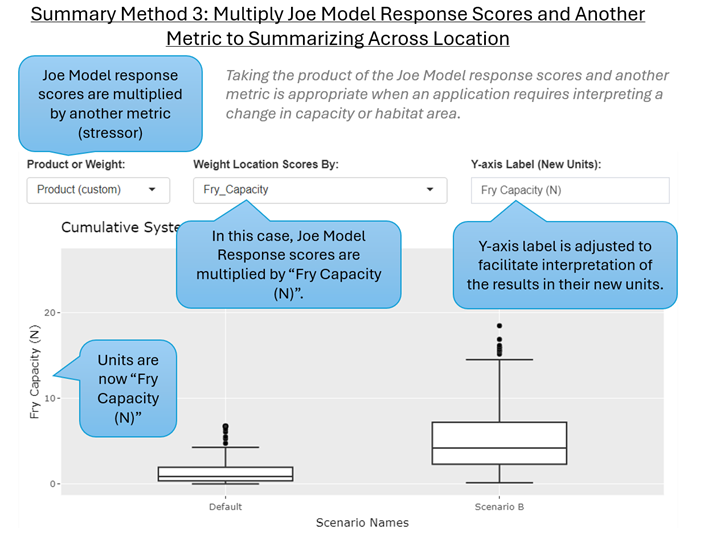
Summary Method 3: Multiply Joe Model Response Scores and Another Metric (e.g., N) to Weight Results Across Locations

Overview: Ultimately, if we can (roughly) estimate habitat capacity (the hypothetical maximum number of individuals) at a location, then we can use the Joe Model system capacity response scores to estimate a change in habitat capacity by taking the product of the Joe Model response scores (0% to 100%, converted to 0 to 1) and an appropriate weighting variable (e.g., habitat capacity (N) by location, calculated as the product of habitat area × density). We can then report the final values in units of the weighting variable (e.g., Predicted Capacity, N). This calculation method provides a myriad of benefits since we can move away from reporting cumulative effect scores as a scale-independent “response percent” and report final values as more concrete units such as habitat capacity in terms of predicted population size (e.g., N) or habitat area (e.g., m²), etc. that are more easily interpretable to a wider audience.

Calculation Method: By taking the product of the Joe Model response score and a weighting variable we convert final scores from a percent to units of the weighting variable. This method is similar to the basic Channel Unit Method described by (Cramer & Ackerman, 2009) to estimate habitat suitability and cumulative effects. Where i is the individual location (channel unit, stream reach, etc.), and the equation represents that change in the capacity across locations as each location is multiplied by all location-specific stressors (scaled from 0 to 1). The sum is taken across all (n) locations and reported as a final value across batch replicates.

Applications:

Estimating a Quantitative Change in Habitat Carrying Capacity: If it is possible to estimate habitat capacity per location (e.g., by multiplying stream area (m²) and an estimate of fish density [hypothetical max N/m²]), we can roughly estimate carrying capacity (N = N/m² × m²). We can then use this metric as the weighting variable in the calculation to report the final score as a change in capacity.
Estimating an Absolute Change in the Weighted Usable Area (WUA): In many instream flow studies, WUA is described as the habitat area in a stream that is considered to be “functional” for a given species/life stage. The WUA value is reported in units of m² but is less than the total stream area. Various Habitat Suitability Index (HSI) curves for depth, velocity, cover, substrate, channel type etc. are multiplied together and then multiplied by the total stream wetted area to calculate the weighted usable area (WUA, m²). We can mimic this calculation in the toolbox if we treat HSI curves as stressors and then take the product of the Joe Model score (0-1) and stream area (m²).

Various other creative methods can be integrated with any metric of interest if there is a rationale to report final values in a specific unit.

The following section describes how to implement each of the different calculation methods in the CEMPRA R-Shiny Application. First, we need to run the Joe Model in the Main Overview tab. After the model is run we can review results in the Scenario Results section. We can also apply weighting in the socio-economic module (Figure 6.7).

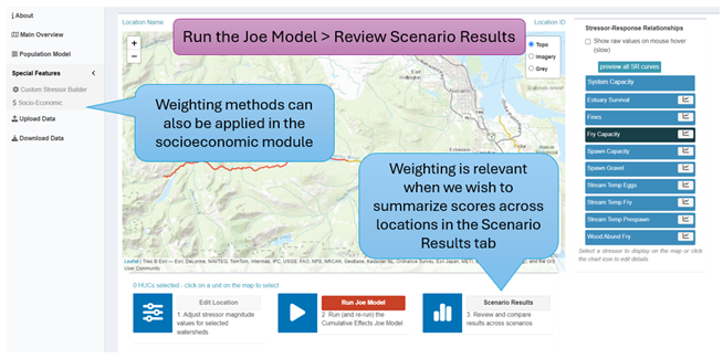
Figure 6.7: Where to apply weighting in the Joe Model.

Next, we can choose to summarize values across locations with either a weighted or unweighted mean (Figure 6.8, Figure 6.9). By default, the Joe Model results are summarized across locations with an unweighted mean (Summary Method 1). By adjusting the ‘Product or Weight’ input box to ‘Weighted Mean’ and selecting a specific weighting variable we can generate results using Summary Method 2 (a weighted mean).

Figure 6.8: Joe Model results summarized across locations with an unweighted mean (Summary Method 1).

Figure 6.9: By adjusting the ‘Product or Weight’ input box to ‘Weighted Mean’ and selecting a specific weighting variable we can generate results using Summary Method 2 (a weighted mean).

We can apply Summary Method 3 ‘Multiply Joe Model Response Scores and Another Metric to Summarize Results Across Locations’ by setting the ‘Product or Weight’ input select box to ‘Product’ (Figure 6.10). We then need to select our metric that will be used as the weighting variables to multiply scores by. Remember to define the new y-axis units appropriately.

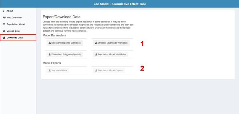
Figure 6.10: Summary Method 3 ‘Multiply Joe Model Response Scores and Another Metric to Summarize Results Across Locations’.

6.7 Download Data

On the Download Data page, you can either download the model input parameter files (i.e., the stressor-response workbook, stressor magnitude workbook, spatial polygons file, and life cycle profile) for offline revisions, or you can directly download the CEMPRA, or Life cycle model outputs for reporting purposes.

Model Parameters: In some circumstances, it may be more convenient to download the stressor magnitude and response Excel workbooks, edit inputs for scenarios offline in Excel or other software and reupload.

Model Exports: The model results can only be exported after the model is run. Export buttons will be disabled until the Joe Model or life cycle model (population model) has been run.

Figure 6.11: Download the Data page of the R Shiny Application. 1) Model parameter files for download. 2) Model output files for download (CEMPRA and life cycle model).